Documentation for xcmocean
xcmocean is a tool that automatically chooses a colormap for your xarray plot and can be used with cf-xarray. The tool will choose a colormap for your plotted variable according to opinionated rules and xarray’s built-in logic will choose whether it will be a sequential or diverging colormap.
Basic Usage
Use xcmocean as an accessor to xarray with .cmo before your .plot() call:
import xarray as xr
import xcmocean
# open an example dataset from xarray's tutorials
ds = xr.tutorial.open_dataset('ROMS_example.nc', chunks={'ocean_time': 1})
# Plot the surface layer (`s_rho=-1`) and 1st time index (`ocean_time=0`)
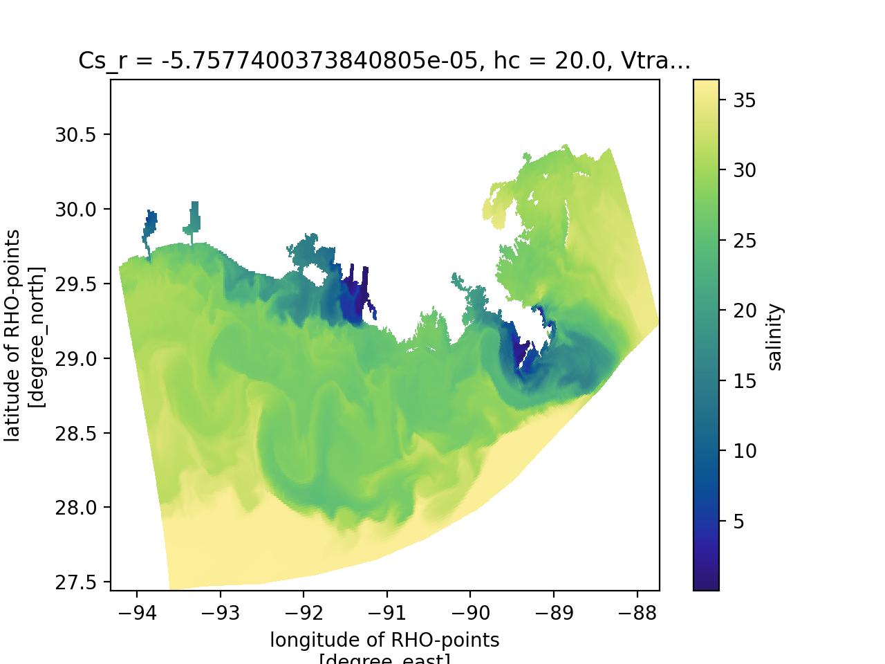
ds.salt.isel(s_rho=-1, ocean_time=0).cmo.plot(x='lon_rho', y='lat_rho')
(Source code, png, hires.png, pdf)

Other Included Functions
The following functions are wrapped in xcmocean for direct use: plot, pcolormesh, contour, and contourf. Here are demonstrations of each using the plot above as an example:
pcolormesh
import xarray as xr
import xcmocean

# open an example dataset from xarray's tutorials
ds = xr.tutorial.open_dataset('ROMS_example.nc', chunks={'ocean_time': 1})

# Plot the surface layer (`s_rho=-1`) and 1st time index (`ocean_time=0`)
ds.salt.isel(s_rho=-1, ocean_time=0).cmo.pcolormesh(x='lon_rho', y='lat_rho')
(Source code, png, hires.png, pdf)

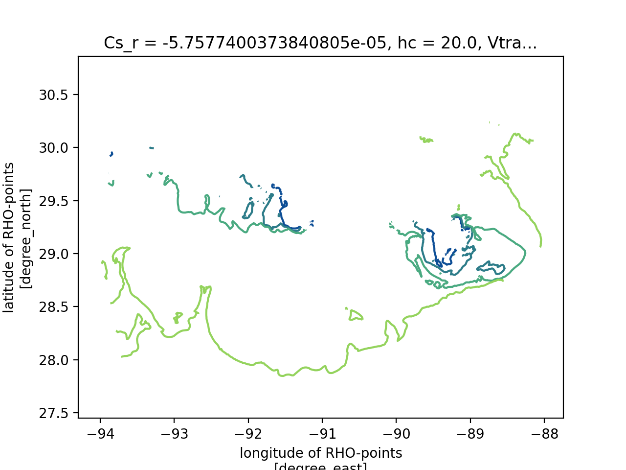
contour
import xarray as xr
import xcmocean

# open an example dataset from xarray's tutorials
ds = xr.tutorial.open_dataset('ROMS_example.nc', chunks={'ocean_time': 1})

# Plot the surface layer (`s_rho=-1`) and 1st time index (`ocean_time=0`)
ds.salt.isel(s_rho=-1, ocean_time=0).cmo.contour(x='lon_rho', y='lat_rho')
(Source code, png, hires.png, pdf)
contourf
import xarray as xr
import xcmocean

# open an example dataset from xarray's tutorials
ds = xr.tutorial.open_dataset('ROMS_example.nc', chunks={'ocean_time': 1})

# Plot the surface layer (`s_rho=-1`) and 1st time index (`ocean_time=0`)
ds.salt.isel(s_rho=-1, ocean_time=0).cmo.contourf(x='lon_rho', y='lat_rho')
(Source code, png, hires.png, pdf)
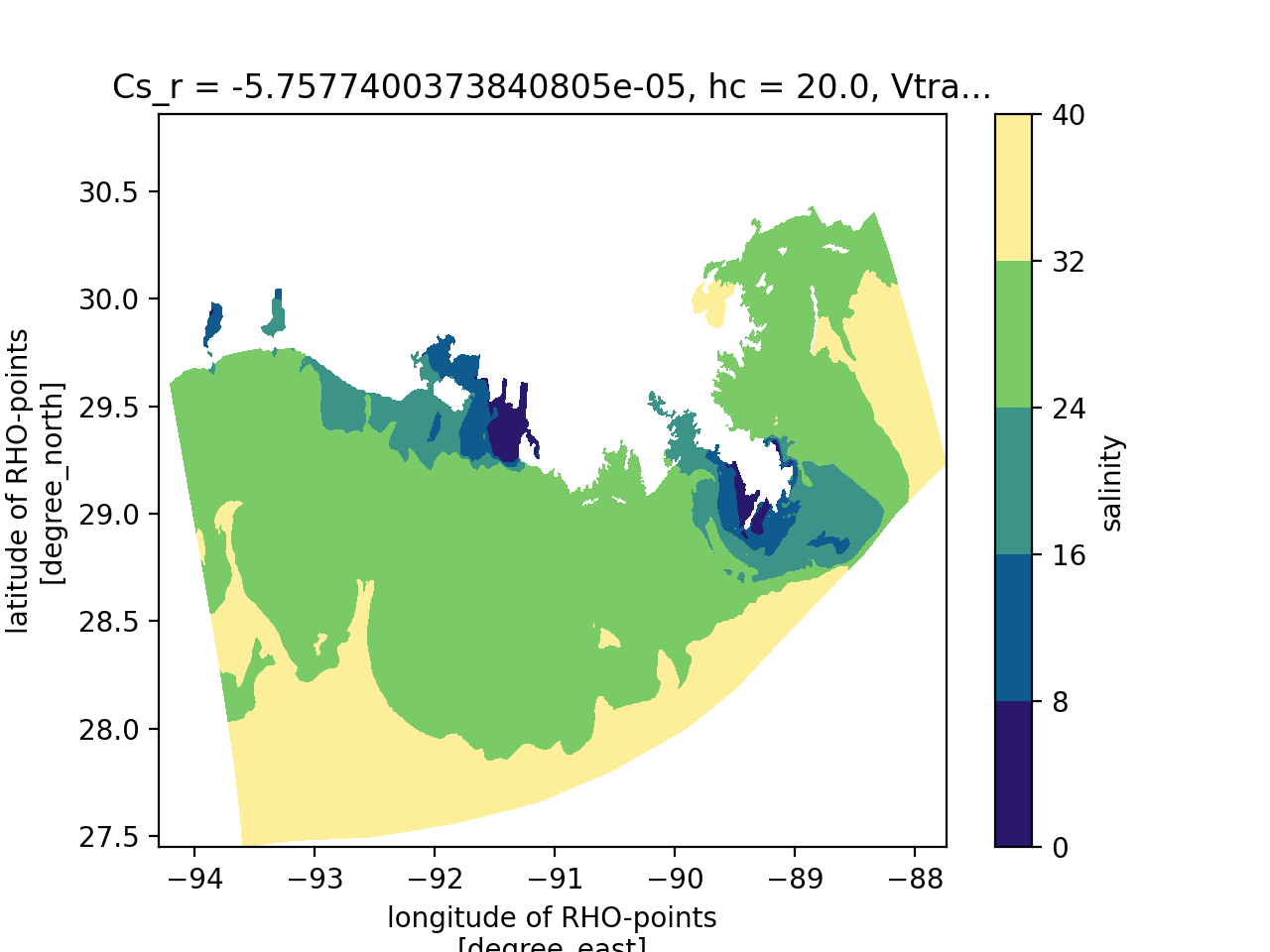
Note that you can input any keyword arguments to the plotting function and they will be simply passed on to the function itself. For example, a filled contour plot can have specified levels input:
import xarray as xr
import xcmocean

# open an example dataset from xarray's tutorials
ds = xr.tutorial.open_dataset('ROMS_example.nc', chunks={'ocean_time': 1})

# Plot the surface layer (`s_rho=-1`) and 1st time index (`ocean_time=0`)
ds.salt.isel(s_rho=-1, ocean_time=0).cmo.contourf(x='lon_rho', y='lat_rho', levels=np.arange(0,40,5))
(Source code, png, hires.png, pdf)
Combining with cf-xarray
xcmocean can be used with cf-xarray for easier, agnostic, consistent handling of dimensions and coordinate names. This is especially convenient for datasets with multiple horizontal grids since with cf-xarray the user doesn’t need to know the name of the grids for a variable. To use these two accessors together, use the same commands as above, but with “cf” before each: cfplot, cfpcolormesh, cfcontour, and cfcontourf. Following is one of the same examples from above. The results are the same, but the function call is a little different:
cfpcolormesh
import xarray as xr
import xcmocean

# open an example dataset from xarray's tutorials
ds = xr.tutorial.open_dataset('ROMS_example.nc', chunks={'ocean_time': 1})

# Plot the surface layer (`s_rho=-1`) and 1st time index (`ocean_time=0`)
ds.salt.isel(s_rho=-1, ocean_time=0).cmo.cfpcolormesh(x='longitude', y='latitude')
Example Variables
The categories of variables available by default are:
In [1]: import xcmocean as xcmo

In [2]: list(xcmo.options.REGEX.keys())
Out[2]:
['temp',
 'salt',
 'vel',
 'freq',
 'zeta',
 'rho',
 'energy',
 'depths',
 'accel',
 'freq2',
 'dye']
A few examples follow:
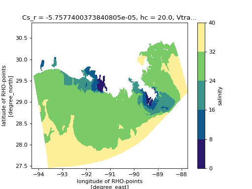
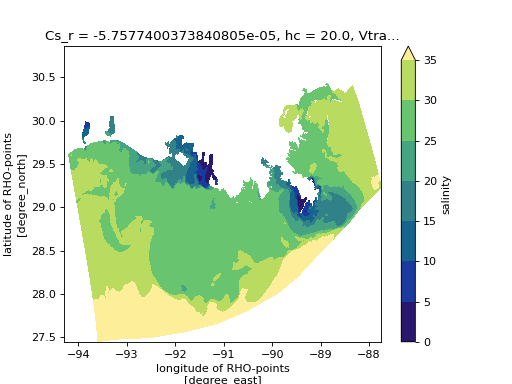
Salinity
import xarray as xr
import xcmocean
import matplotlib.pyplot as plt

fig, axes = plt.subplots(1, 2, figsize=(15,5), sharey=True)

# open an example dataset from xarray's tutorials
ds = xr.tutorial.open_dataset('ROMS_example.nc', chunks={'ocean_time': 1})

# Plot the 1st time index (`ocean_time=0`) and surface layer (`s_rho=-1`)
var = ds.salt.isel(ocean_time=0, s_rho=-1)

# Sequential
var.cmo.cfplot(x='longitude', y='latitude', ax=axes[0])

# Create a diverging dataset for demonstration
(var - var.mean()).cmo.cfplot(x='longitude', y='latitude', ax=axes[1])
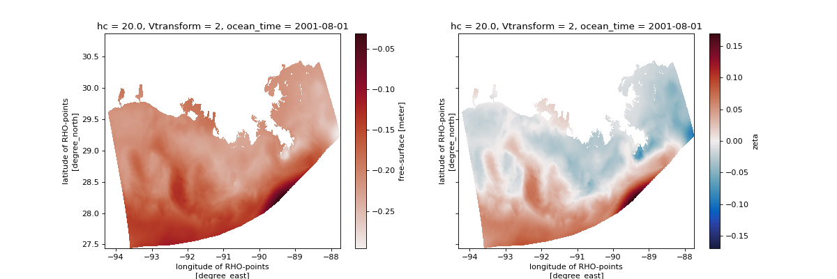
Free Surface Height
import xarray as xr
import xcmocean
import matplotlib.pyplot as plt

fig, axes = plt.subplots(1, 2, figsize=(15,5), sharey=True)

# open an example dataset from xarray's tutorials
ds = xr.tutorial.open_dataset('ROMS_example.nc', chunks={'ocean_time': 1})

# Plot the 1st time index (`ocean_time=0`)
var = ds.zeta.isel(ocean_time=0)

# Sequential
var.cmo.plot(x='lon_rho', y='lat_rho', ax=axes[0])

# Create a diverging dataset for demonstration
(var - var.mean()).cmo.plot(x='lon_rho', y='lat_rho', ax=axes[1])
(Source code, png, hires.png, pdf)

Bathymetry
import xarray as xr
import xcmocean
import matplotlib.pyplot as plt

fig, axes = plt.subplots(1, 2, figsize=(15,5), sharey=True)

# open an example dataset from xarray's tutorials
ds = xr.tutorial.open_dataset('ROMS_example.nc', chunks={'ocean_time': 1})

# variable is 2d
var = ds.h

# Create a sequential dataset for demonstration
var.cmo.cfplot(x='longitude', y='latitude', ax=axes[0])

# Create a diverging dataset for demonstration
(var - var.mean()).cmo.cfplot(x='longitude', y='latitude', ax=axes[1])
How it works
xcmocean works by searching the DataArray variable name and attributes for clues about what type of variable it is, then matching that with a set of built-in options.
Check identified variable type
Determine the variable type or category that has been identified by xcmocean with the following:
In [3]: import xarray as xr

In [4]: ds = xr.tutorial.open_dataset('ROMS_example.nc', chunks={'ocean_time': 1})

In [5]: print(ds.h.cmo.vartype())
depths
Get more information by including verbose=True:
In [6]: print(ds.h.cmo.vartype(verbose=True))
bathy|depths|bathymetry matches bathymetry at RHO-points in attributes
depths
Return the sequential colormap and name:
In [7]: ds.salt.cmo.seq, ds.salt.cmo.seq.name
Out[7]: (<matplotlib.colors.LinearSegmentedColormap at 0x7f328b83a7d0>, 'haline')
Return the sequential colormap and name:
In [8]: ds.salt.cmo.div, ds.salt.cmo.div.name
Out[8]: (<matplotlib.colors.LinearSegmentedColormap at 0x7f3289dcd890>, 'diff')